What is Flow Debt?

+Daniel Vacanti's excellent treatise on Actionable Agile Metrics [vaca] introduces a term that may be unfamiliar, even to those with an interest and experience in managing flow systems. The term is Flow Debt - for a definition and explanation read on.

My own particular interest in flow systems is the management of agile software development teams, usually using some variant of Scrum and/or Kanban, and other agile practices such as test-driven (or automated-test intensive) build-test-deploy processes. However the discussion is relevant in many other domains, such as one I've recently been involved in discussing, the flow of patients through diagnosis, treatment and convalescence in healthcare systems.

In managing these systems we need ways to look at the mass of data that emerges from them to focus on the useful information rather than the noise; information in particular that indicates when intervention is appropriate to improve flow, and when the attempt would be as futile as trying to smooth the waves on an ocean. Flow systems in knowledge work contain variability. That variability, within certain bounds (much wider bounds than in manufacturing for example), is desirable to allow innovation, responsiveness and minimising wasteful planning activities.

In this context Flow Debt is a measure that provides a view of what is happening inside our system. This is in contrast with other important measures such as Throughput (Th) and the time an item stays in the process (I call this "Time in Process", TiP [macc], though other terms may be used). These measures provide information only after items have left the system, which may be too late to avoid problems accumulating.

Having Flow Debt roughly translates as: delivering more quickly now at the cost of slower times later. It is calculated by comparing the time since the number of arrivals into the systems was equal to the current number of deliveries with the average time in the process for the most recent deliveries. It is easiest to visualise this on a Cumulative Flow Diagram.

At the point highlighted in the the diagram it is a little over 2 weeks since the cumulative number of items entering the system equalled the cumulative number of deliveries on that date. If the items were delivered in the precise order they arrived, and if all the items were delivered (neither assumption is true!), then we would be able to say that the time the last item spent in the process was also a little over 2 weeks. Furthermore if arrivals and deliveries were smooth over the period, the Average Time in Process for the items would also be this same time.

What was the actual Average Time in Process though? Well you can't read this off the diagram. You have to look at the average TiP for the items delivered in the recent period. Each one has a known TiP, so take the average of them. Exactly how long the period you select for this average is up to you - a day or a week seems reasonable. The shorter the period you take the more noise there will be in the signal. Take too long a period though and there is insufficient time to act on the information. 

With this information we can calculate Flow Debt using Dan's method[vaca]:

Flow Debt = (Time since number of arrivals equalled deliveries) - Average TiP

If you plot this quantity for the data above you get a graph like this. Note I've reversed the sign on this graph to show Flow Debt as negative.

The plot of Flow Debt in this case is quite normal showing a fluctuation around zero and maxima and minima of around the value of the average TiP for the whole period. If you plotted the same data with a monthly average, most of this fluctuation would disappear. I certainly wouldn't want managers rushing down to this team to radically change their process!

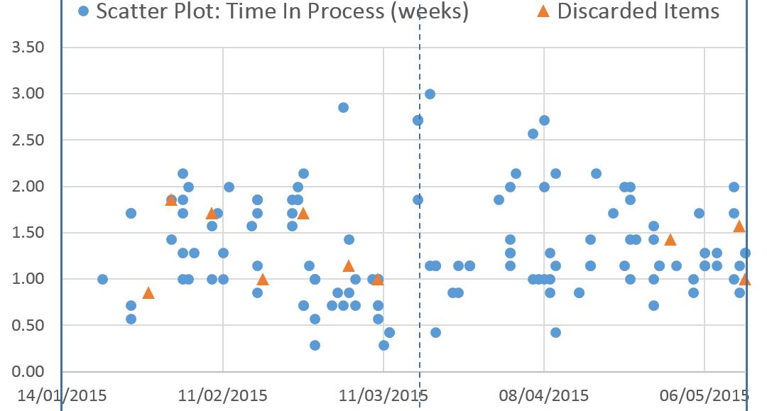
There is one point highlighted which is interesting, where the Flow Debt goes from highest debt to highest credit in a few days. What do you think is going on here? Well, if you go back to the informal definition of Flow Debt (delivering more quickly now at the cost of slower times later), we should surmise that before this point the delivered items had been in the process for only a short time. Those delivered at or after this point had a longer time in the process. That's exactly what happened, as the Control Chart below shows.

Another useful indicator here is the "average age" of the work in progress. Here is the plot of that and you can see the significant drop in this metric at the same point.

Just by way of balance let's look at another data set of a team delivering software much less frequently, where their work in progress is increasing over the process, and where the items are not being delivered in age order. All these factors are likely to effect the efficiency and predictability of the flow system... and this is borne out by their plot of Flow Debt.

Seeing a plot like this is a indication to management (and flow management specialists in particular) to take a much closer look at the process being used here.

References

• [macc] Maccherone, Larry. Introducing the Time In State InSITe Chart. LSSC. (2012)
• [vaca] Vacanti, Daniel S. Actionable Agile Metrics for Predictability: An Introduction, LeanPub. (2015)

Beyond Control Charts and Cumulative Flow Diagrams

Control Charts (CCs) and Cumulative Flow Diagrams (CFDs) are powerful ways to display information about a flow system, such as a Scrum or Kanban development process. Unfortunately the very fact that the charts display so much information means that it is often difficult to extract specific information from them. That is why it's useful to also plot some of the key attributes of the systems on their own - this allows us to look at these aspects specifically, alongside the rawer view of the data that you get from CCs and CFDs.

The graphic on the right shows a number of diagrams all of which were derived from very simple data about each item that flowed through this system:

• when it arrived into the system; 
• when it departed the system; and
• whether the item was "delivered" or "discarded".

Note: I use the term "discard" here as a general term to include an exit from the system at any point in the system and for any reason. It includes aborting/abandoning the item after commitment, as well as postponing the item by moving it back to a part of the process upstream from the system under study. For the definition of this and other terms used here please see this Glossary.

The first diagrams in the graphic is the Control Chart - actually this is simply a scatter plot of the time each item stays in the system under study. I refer to this as "Time in Process - TiP - or alternatively "Time in _______" where the blank stands for whatever the process or part of the process is under study. For example it could be the Time in Preparation, Time in Development, Time in Acceptance, etc. The scatter plot highlights (in orange) the items which were not "delivered".

Below it is the CFD. Unlike some very stripy versions, this one has only 3 bands (as limited by the input data), corresponding to arrivals, all departures (including discards), and deliveries.

The remaining diagrams all highlight one or more aspects of the same data. Firstly the terms from Little's Law:

1. Average Delivery Rate. This is measured in items per week, and the average is taken over 1 week. Note this only shows actually delivered items. Alternatively a plot of "Throughput" could have been used which includes all items that have passed through the system.
2. Average Time in Process (TiP). This is measured in weeks and again the average is taken over 1 week.
3. Average Work in Progress (WiP). This is measured in number of items, again averaged over one week. Care must be taken when calculating average WiP for a day, particularly on days when an item arrives in or departs from the system, to ensure that it is consistent with the calculations of average TiP.

In addition to these standard quantities from Little's Law a number of flow balance metrics are shown. These are:

4. Net Flow. Simply the difference between the number arriving and departing over the previous week.
5. Delivery Bias. This is a measure of the degree to which Delivery Rate is higher or lower than would be predicted by Little's Law for the given period (1 week in this case). If it is non-zero it indicates away from stability. Further discussion of this quantity is found here.
6. Flow Debt/Credit. This is a measure of the degree to which the average TiP varies from that predicted by the CFD. This also indicates a degree of instability if it varies significantly from zero. See Dan Vacanti's book [vaca] for further discussion.
7. Age of WiP Indicator. This compares the average age of the WiP with half the average Tip. It is another indicator of imbalance.

Recently I have been discussing these four quantities with colleagues and with Troy Magennis and Dan Vacanti as they show promise for predicting significant changes in the TiP, a very important aspect of the effectiveness of the system.

A spreadsheet containing the means to generate these diagrams from your data will shortly be made available from gitHub. Watch this space!

References

• [vaca] Vacanti, Daniel S. "Actionable Agile Metrics for Predictability: An Introduction". LeanPub. (2015)

Postscript on Throughput and Delivery Rate

Most people use Throughput and Delivery Rate in Kanban systems as synonyms - including myself up to this point. I've changed my view however.

The canonical form of Little's Law in Kanban is as follows:

Delivery Rate = WiP / Lead Time    [ande] 

even though these days I more frequently express it this way:

Throughput = WiP / TiP 

Surely these two ways of writing the equation are entirely equivalent aren't they? Well maybe not.

Note: All these terms are defined in my Glossary Proposal (which has recently been updated to include the definition of Throughput). Feedback, comments and references to publications using the terms defined are welcomed and encouraged.

Throughput is the term +Daniel Vacanti uses (among many others), particularly in his excellent new book Actionable Agile Metrics [vaca], and it got me thinking about one of the problems with using Delivery Rate: what about the items which are not delivered but are discarded? If there are a significant number of these Little's Law as expressed in the first equation will not apply, unless we exclude discarded items from calculations of the historical averages for WiP and TiP. All very well except the WiP limits - a crucial control for Kanban systems necessarily contain items that may be discarded in the future.

Without trying to solve this problem, but rather clarify the terminology we use to describe it, I think it is useful to have differing definitions for the 2 terms:

Delivery Rate is the rate at which work items exit the system in a "complete" state (i.e. just delivered items)

Throughput is the rate at which work items exit the system whether discarded (this includes those which move back in the process to a state prior to the system under consideration) or completed (i.e. both delivered and discarded items)

Let me know if you find this distinction useful. Your feedback is essential in honing the Glossary Proposal to one that everyone finds helpful and acceptable.

References

• [ande] Anderson, David J. Kanban, Blue Hole Press. (2010)
• [vaca] Vacanti, Daniel S. "Actionable Agile Metrics for Predictability: An Introduction". LeanPub. (2015)

Little's Inequality

The interesting thing about Little's Law, in spite of its very general applicability, and in certain cases mathematical certainty, there are many cases when it simply does not hold true. In those cases it's not so much Little's Law as Little's Inequality. Could the fact that specific instances of data do not follow Little's Law actually give us useful information about our Kanban and Scrum systems and point to the right kind of interventions to manage and improve their flow? That's what this blog is about.

Flow Metrics for a Kanban System over time
(WiP, TiP, DR, Delivery Bias, Net Flow)

In 1961 John Little published his proof of this general queuing theory equation [litt]:

L=λW 

L is the average number of items in the queue, λ is the average arrival rate, and W the average wait time

Since that time Little's Law has found numerous applications in the study of general flow systems from telecommunications to manufacturing, including in Kanban systems. Because throughput or delivery rate is the more significant attribute for management of such systems (and on average it is approximately equal to arrival rate), it is often expressed as follows:

Delivery Rate = WiP / TiP 

The overline indicates the arithmetic mean, WiP is the number of items in the system, and TiP the "time in process" from entering to leaving the system under consideration. See this Glossary for further explanation of the meaning of TiP, versus Lead Time or Cycle Time (and why I don't use Cycle Time!).

However when we look at data from actual Kanban systems, where the averages are over relatively short periods (say a week or a month), or where average arrival rate does not equal average delivery rate, it is Little's Inequality that applies, not his Law. Juggling the terms above we can express it in this way:

Delivery Rate – ( WiP / TiP ) ≠ 0    ("Little's Inequality")

This is because if the system itself is trending in some way (technically the system is not stationary), or if the scope of the averages is not so wide that every item that entered has left the system - usually both these conditions are true for the periods we wish to analyse - then Little's Law does not apply exactly.

That might seem to imply Little's Law is not useful to us. However the degree to which the law is not true is very relevant and does give us important management information:

Delivery Rate – ( WiP / TiP ) < 0    More work is being taken on than is being delivered

Delivery Rate – ( WiP / TiP ) = 0    The system is balanced

Delivery Rate – ( WiP / TiP ) > 0    More is being delivered than new work being taken on

This looks like actionable data for managing flow in Kanban Systems - a number that shows bias in the system towards (or away from) delivering. Let's look at the set of graphs in the figure above that demonstrate this. The data set is from +Troy Magennis's SimResources website and uses his data, spreadsheet and some of the graphs he provides to assist with his forecasting models[mage]. You can find more about Troy's work at FocusedObjective.com and also download these spreadsheets to explore what your data reveals about your Kanban or Scrum systems.

Firstly the figure shows graphs of the 3 main variables in Little's Law: WiP, TiP and Delivery Rate, The next graph is a plot of Little's Inequality - labelled Delivery Bias, showing whether it is greater or less than zero at any point in time. Note that the formula above is normalised relative to the overall average delivery rate for the whole dataset (AvDR) so that the range (in this case between -1 and +1) is comparable with other datasets. The final graph in the set shows Net Flow, the difference between items completed and started - it is one of the metrics included in Troy's spreadsheet and it again provides a view of how balanced the system is.

As expected the graphs show a strong correlation between Net Flow and Little's Inequality for most of the range. Clearly if we're starting more than we're finishing we should expect both the inequality and the Net Flow to be negative. What's interesting is where they don't correspond, and why. Look at weeks 2015-11 and 2015-12. Why in week 11 are we finishing more than starting and yet we still have a negative value for Little's Inequality? The clue is in the TiP for these weeks. In week 11 the average TiP is much lower than in week 12. Perhaps this indicates the items closed that week were smaller in size - or maybe they were "expedited" at the expense of other items in progress. When the items that had been in process longer are closed the following week, Little's Inequality indicates more strongly that balance is being restored.

Little's Inequality as expressed above focuses on Delivery Rate, hence the label Delivery Bias. It could be re-expressed to focus on Time In Process as follows:

TiP – WiP / Delivery Rate ≠ 0     

This metric might be labelled Time in Process Bias. We want TiP values to be as low as possible, but a negative value of this metric is likely to indicate an issue to address, since it would indicate that the TiP of the work in progress is likely to be longer than the items recently delivered.

The time an item stays in the process is also the focus of a new metric from +Daniel Vacanti recently published in his Actionable Agile Metrics [vaca] (see also ActionableAgile.com). He also looks at the degree to which a given system follows an ideal flow through a metric he calls "Flow Debt" (roughly translated as delivering more quickly now at the cost of slower times later). Dan prefers the term Cycle Time to Time In Process and so defines Flow Debt as the difference between the "Approximate Average Cycle Time" (AACT) as observed on a Cumulative Flow Diagram and the "Average Cycle Time" (ACT). Comparing these 2 items gives an idea of whether Flow Debt  is being created or not. Flow Debt is accumulating when AACT>ACT. You can calculate AACT by looking at the time since the cumulative arrivals into the system equalled the current cumulative deliveries. ACT is calculated from the arithmetic mean of the actual times for delivered items in the period. Again the degree to which these quantities do not match indicates the degree to which the system is out of balance.

All these metrics - Little's Inequality (or Delivery Bias), Net Flow and Flow Debt - provide insight into the behaviour of Kanban systems based on the degree to which the system follows Little's Law over the period of study. Further experimentation and experience will show the best ways to use them in concert and the best ways to visualise the flow characteristics of the systems and how to intervene to improve them.

If you have data which you would like to analyse using these metrics do let me know. I'm happy to share spreadsheets and advice with anyone who contacts me. Equally check out Troy Magennis's and Dan Vacanti's web sites referenced above for more tools and insights.

References

• [litt] Little, J. D. C. "A Proof of the Queuing Formula: L = λW," Operations Research, 9, (3) 383-387. (1961) 
• [mage] Magennis, T. "Forecasting and Simulating Software Development Projects: Effective Modeling of Kanban & Scrum Projects using Monte-carlo Simulation", FocusedObjective.com. (2011)
• [vaca] Vacanti, Daniel S. "Actionable Agile Metrics for Predictability: An Introduction". LeanPub. (2015)

Glossary Proposal

One of the problems Kanban practitioners have faced over the past several years is the lack of agreement of the terminology to use to describe flow systems. This in turn has led to confusion in both those learning the method and those implementing tools to support it. This blog has made a few previous attempts to disambiguate common terms (see discussions of Cycle Time for example). Mike Burrow's Glossary of Terms, [burr] reproduced on the Lean Kanban University site [lkun] is also very useful, though it does not give guidance on which terms to use when applying Little's Law to sub-processes in a more complex Kanban system. 

This article is another foray into this minefield and is principally a proposal for the definitions of commonly used terms relating to Little's Law, particularly seeking terms applicable in complex flow systems and sub-processes within such systems. It is an invitation to others in the community to endorse these definitions, or propose alternatives. Let's not go another seven years with this unresolved!

Note: This is a work in progress and will be updated from time to time in response to feedback from other authors and practitioners.

The Kanban Method is a process improvement approach based on understanding knowledge work as a flow system. The life cycles of the "work items" in such flow systems are analysed and improvements to the process are made based on observable positive change. So let's start with Little's Law since it is the first basis of understanding flow systems. For a given system it may be defined as follows [litt]:

Arrival Rate = WiP / TiP     
where the overline indicates the arithmetic mean in a "stationary" or other compliant system.

Arrival Rate
Measured in: work items per unit of time (seconds, hours, days. working days, etc.)
Definition: The number of units entering the system per unit of time. The work item must be defined for the metric to be meaningful (e.g whether a User Story, Feature, Case, Initiative, Physical Item, Episode, Request, etc.). Little uses Arrival Rate in his definition of the law. In a "compliant" system the average rate of items arriving in the system and leaving it must be equal:

Arrival Rate = Throughput 

Throughput and Delivery Rate are usually treated as synonyms in Kanban systems. However if a distinction is made between delivered and discarded items (essential if we are to understand productivity effectively), a distinction should also be made between these terms. Since items may be either delivered or discarded:

Throughput = Delivery Rate + Discard Rate 

If the Discard Rate is not significant or we exclude discarded items, we can use the common formulation of Little's Law found in Kanban system analysis:

Delivery Rate = WiP / TiP

If the Discard Rate is significant, the historical values of WiP should include only those items that have been delivered and TiP should be the time in process for delivered items only, not discarded ones. (Alternatively use Throughput and ensure that the time in process for discarded items is included.)
Related terms: Throughput, Delivery Rate, Discard Rate, Discard, Abort
References: [ande], [burr], [litt], [vaca]

Throughput
Measured in: work items per unit of time
Alternatives: Throughput Rate, Departure Rate, Processing Rate [rein]
Definition: The number of work items exiting from the system per unit of time, whether delivered or discarded. See also: Postscript on Throughput and Delivery Rate.
Related terms: Delivery Rate, Arrival Rate, Discard Rate
References: [vaca]

Delivery Rate
Measured in: work items per unit of time
Alternatives: Completion Rate
Definition: The number of work items emerging complete from the system per unit of time, This is a key metric to understand the productivity of the system.
Related terms: Arrival Rate, Discard Rate, Throughput
References: [ande], [burr]

Discard Rate
Measured in: work items per unit of time
Definition: The number of work items discarded before completion per unit of time. In typical Kanban systems this metric may be significant relative to Arrival Rate, particularly where the "2 stage commit" is used to prepare but not necessarily complete options. Discard is a general term for abandoning a work item. More specifically to Abort a work items means to discard the item after the Commitment Point in a development system
Related terms: Arrival Rate, Throughput, Delivery Rate, Commitment Point, Abort, Discard

Commitment Point
Measured in: not a metric, a specific point in a defined process
Definition: In a development system process, it is the point at which a commitment is made to develop the work item. Before this point work done supports the decision whether or not to develop the item.
Related terms: Abort, Discard

Abort
Measured in: not a metric, an action
Definition: To Discard a work item after the Commitment Point.
Related terms: Commitment Point, Discard

Discard
Measured in: not a metric, an action
Definition: To stop work on an item and remove it from the process. Note that an item is "discarded" in this sense even if it might be worked on in the future, for example if the work item is moved back to a queue prior to the system/sub-process under consideration. The term is not specific about when in the process the item is discarded, however in a development system process it may apply to items discarded prior to the Commitment Point, since after this point the term Abort is applicable.

Related terms: Abort, Commitment Point

WiP, Work in Progress
Measured in: work items
Definition: The number of work items which have entered the system but which are not yet either completed or discarded.
Related terms: Arrival Rate, Throughput, Delivery Rate, TiP

References: [ande], [burr], [hopp], [marc], [rein]

TiP, Time in Process

Measured in: units of time

Alternatives: Cycle Time (but see cautionary note below), Lead Time (when referring specifically to the time in process in a Kanban development system from the Commitment Point to delivery), Throughput Time [modi], Time In System [rein]

Definition: The time that a work item remains in the system or sub-process under consideration prior to being either completed or discarded. This is the key metric in understanding the time to delivery of a system. More specific terms may be derived by replacing "Process" with the particular part of the process of interest, for example "Time in Development". As with all the terms in Little's Law the scope of the system or sub-process under consideration must be well defined to ensure they are meaningful.

A key reason for recommending this term is that it sidesteps the "Cycle Time versus Lead Time" debate which shows no sign of resolution within the communities that use these terms.
Related terms: Cycle Time, Lead Time, Touch Time, Takt Time
References: [macc]

Cycle Time
Measured in: units of time

Alternatives: For CT1 (defined below) use its reciprocal - Delivery Rate; for CT2 use TiP or (where applicable) Lead Time

Definition: The time taken for a "cycle". This is a very ambiguous term which should not be used in Kanban without qualification. Examples of where it is commonly used in the literature are:

• In a factory: the time between completed units exiting the system [chew], [like], [marc], [woma]
• For a queue: the time an item remains in the queue [litt]
• For an airport security control: the (average) time between two items completing the process [modi]
• For a work station or machine: the time between completed parts exiting the station [chew], [like], [marc], [woma]
• For a worker/team: the time between starting and completing an item [hopp], [modi], [rein], [vaca]
• For a project/team: the time between deliveries of completed items [beck]

It is incorrect to use the term for any period which is not contiguous, e.g. Touch Time or aggregated time in a column. Unfortunately such usage may be found in some tool implementations.

Broadly speaking there are two categories of usage for Cycle Time which may be referred to as CT1 and CT2. CT1 is the time between successive items emerging from a station or system. CT2 is the time an item takes from entering the system to leaving it. It is left to the reader to decide which of the examples above are CT1 or, CT2. Note that there is a special case (when WiP=1) where CT1=CT2. Unfortunately this just tends to confuse people further, especially when the example given to define the term is an example where WiP=1!

Where Cycle Time is used in the Kanban community, its definition "generally" coincides with that of Lead Time for Kanban development systems given below.

Author's Note: Since there is no universally accepted definition of what Cycle Time means in a flow system, the term should simply be avoided.
Related terms: TiP, Lead Time, Touch Time, Takt Time
References: [beck], [burr], [chew], [hopp], [litt], [marc] [modi], [rein], [roth], [vaca], [woma]

Lead Time
Measured in: units of time
Definition: In general usage, Lead Time means the time from the request for an item to the delivery of the item (this may simply be the time to get an item from stock or the time to specify, design, make and deliver an item). However its usage in Kanban development systems is more specific. It indicates the time from the Commitment Point to the delivery. For this to be useful the commitment and delivery points must be made explicit.
Note there remains some ambiguity in this term and I would recommend using TiP in most circumstances, and certainly when analysing sub-processes in a larger flow system. If you use Lead Time, qualify it if necessary (e.g. Development Lead Time and ensure that you define the meaning that you wish to be assigned to it in your context.
Related terms: TiP, Cycle Time, Touch Time, Takt Time

References: [ande], [burr], [marc]

Touch Time
Measured in: units of time
Alternatives: Value-Creating Time
Definition: The sum of all the times during which a work item is actively being working on (excluding wait times, for example being held in stock or in queues).
Related terms: TiP, Cycle Time, Lead Time, Takt Time

References: [modi], [woma]

Takt Time
Measured in: units of time
Definition: The projected customer demand expressed as the average unit production time (i.e. the time between the completion of work items) that would be needed to meet this demand. It is used to synchronise the various sub-processes within the system being designed to meet demand without over or under production.
Related terms: TiP, Cycle Time, Lead Time, Touch Time

References: [marc], [rike], [woma]

Flow Efficiency
Measured in: %
Definition: The ratio of the time spent working on an item (Touch Time), to the total time in process (TiP), i.e.:

Flow Efficiency = Touch Time / TiP

Related terms: Resource Efficiency

References: [modi]

Resource Efficiency
Measured in: %
Definition: The ratio of the time a resource (for example a person!) is actively working on a work item, to their total available time.
Related terms: Flow Efficiency
References: [modi]


References

• [ande] Anderson, David J. Kanban, Blue Hole Press. (2010)
• [beck] Beck, Kent and Martin Fowler, Planning Extreme Programming, Addison Wesley (2000)
• [burr] Burrows, Mike. Kanban from the Inside, Blue Hole Press. (2014)
• [chew] Chew, W. Bruce, Harvard Business School Glossary of Terms [as referenced by Fang Zhou]. (2004)
• [hopp] Hopp, W.J and M. L. Spearman, Factory Physics, 3rd ed., McGraw Hill, International Edition. (2008)
• [like] Liker, Jeffrey K. The Toyota Way, McGraw Hill. (2004)
• [litt] Little, J. D. C and S. C. Graves. Little's Law, pp 81-100, in D. Chhajed and TJ. Lowe (eds.) Building Intuition: Insights From Basic Operations Management Models and Principles. doi: 10.1007/978-0-387 -73699-0, (c) Springer Science + Business Media, LLC. (2008)
• [lkun] Lean Kanban University. Glossary of Terms, from Kanban from the Inside, Mike Burrows. (2014)
• [marc] Marchwinski, C. et al Eds, 4th ed, Lean Lexicon, a graphical glossary for Lean Thinkers. (2008)
• [macc] Maccherone, Larry. Introducing the Time In State InSITe Chart. LSSC. (2012)
• [modi] Modig, N. and P. Åhlström, This is Lean, Rheologica Publishing. (2013)
• [rein] Reinertsen, Donald G, The Principles of Product Development Flow, Celeritas Publishing. (2005) 
• [roth] Rother, Mike and John Shook, Learning to See: Value Stream Mapping to Add Value and Eliminate Muda, Lean Enterprise Institute. (2003)
• [vaca] Vacanti, Daniel S. Actionable Agile Metrics for Predictability: An Introduction, LeanPub. (2015)
• [woma] Womack, J. P. and D. T Jones, Lean Thinking, Simon and Schuster. (1996, 2003)

Growing Kanban in Three Dimensions

Kanban systems can work at different scales and in widely different contexts. Indeed any organisation that delivers discrete packages of value ("work items") and which is interested in maximising the value and timeliness of its delivery, can analyse and improve its performance using the Kanban method. 

Kanban systems can grow - in fact in most cases it's much better that they grow than a massive process change is made suddenly across a whole organisation. "Big bangs" tend to be quite destructive, even if they could clear the way for something new. There are three dimensions in which Kanban systems grow:

• Width-wise growth: encompassing a wider scope of the lifecycle of work items than the typical "to do - doing - done" a single division of the process. It can cover from the idea to real value - or "concept to cash", though cash may come before or after the realisation of real value.
• Height-wise growth: by considering the hierarchy of items that make up valuable deliveries, each level of the hierarchy having differing flow characteristics. (This dimension use the "scale-free" nature of Kanban, the same principles and practices apply whatever the size of the work item.)
• Depth-wise growth: not only depth of understanding but depth of penetration through the full set of services required by the organisation to deliver value. (Sometimes referred to as "Scaling by not scaling" or "service-oriented Kanban", the approach here connects multiple services at the same level through feedback loops that balance the capacity of the various kanban systems.)

We'll look at each of these dimensions in upcoming articles. Which dimension to grow first will depend on context and the motivations for change. Any change needs to pay for itself with improvements in the flow of value, so asking "why?" is a more important first question than "what?".

When you come across a good idea ("agile" in general springs to mind at this point) it is very tempting to sweep away whatever you were doing before you were converted to the new idea, and start doing it everywhere. It should not come as a surprise to those who do this, that very soon a new idea will come along. With the poor results from mass conversion to the caricature of the original idea you adopted, the same cycle will be repeated. Instead grow the changes organically.

Try this: start small; understand the ideas as you assimilate them; grow what works and understand what doesn't work; work out why. Success will follow.

Acknowledgement: Thanks to +Pawel Brodzinski for the discussions on Portfolio Kanban... and one of the graphics on the top floor of the above diagram.

Earned Value Management and Agile Processes

I've recently been working with a client whose customer requires project reporting using Earned Valued Management metrics (EVM). It made me realise that, since they are also wishing to use agile methods, a paper I wrote back in 2008 could be relevant to them, and maybe a few others. When I looked for it online it was no longer available, so I thought I'd remedy that here. You can access the paper by clicking this link: EVM and Agile Processes – an investigation of applicability and benefits.

EVM is a technique for showing how closely a project is following both its planned schedule and planned costs. It's a superior method to simply reporting time and cost variance, since if the project has slipped but also underspent you cannot tell from the simple variances the degree to which the underspend has caused the slippage. EVM's cost efficiency and schedule efficiency (nothing to do with efficiency by the way!) can tell you this.

However agile methods do not have a fixed scope during their lifecycle and this can make EVM reporting effectively meaningless. The paper explains a technique for using the substitutability of User Stories, estimated in points, for overcoming this problem. If this is relevant to your business environment, I hope you find it useful.

Agile EVM has continued to develop since this paper and you can find more details and further references in the Wikipedia entry here: Earned value management: Agile EVM.

Citation: Andy Carmichael (2008). EVM and Agile Processes – an investigation of applicability and benefits, The 2nd Earned Value Management Conference, NEC, Birmingham UK, 12 March 2008.
Project Manager Today Events. www.pmtoday.co.uk.

Does your Definition of Done allow known defects?

Is it just me or do you also find it odd that some teams have clauses like this in their definition of done (DoD)?

Done... or Done-But?

... the Story will contain defects of level 3 severity or less only ...

Of course they don't mean you have to put minor bugs in your code - that really would be mad - but it does mean you can sign the Story off as "Done" if the bugs you discover in it are only minor (like spelling mistakes, graphical misalignment, faults with easy workarounds, etc.). I saw DoDs like this some time ago and was seriously puzzled by the madness of it. I was reminded of it again at a meet-up discussion recently - it's clearly a practice that's not uncommon.

Let's look at the consequences of this policy. 

Potentially for every User Story that is signed off as "Done" there could be several additional Defect Stories (of low priority) that will be created. It's possible that finishing a Story (with no additional user requirements) will result in an increase in the Product Backlog size! (Aaaagh...) You're either never going to finish or, more likely, never going to fix those Defects in spite of all the waste that will be generated around recording, estimating, prioritising and finally attempting to fix the defects (when the original developer has forgotten how he coded the Story, or has been replaced with someone who never knew it in the first place).

What should happen then? 

Clearly the simple answer is that if you find a bug (of whatever severity) before the Story is "Done", fix it. You haven't finished until it works - just avoid double-think like I've finished it even though the product now contains new defects.

Can there be exceptions to this?

Those who think quality is "non-negotiable" would probably answer "No", but actually (whether acknowledged or not) we all work with a concept of "sufficient quality". It is inherent in ideas like "minimum viable product" and "minimum marketable feature". Zero defects is a slogan not a practicable policy for most product developments. Situations where we find defects that are hard to fix when working on a User Story, bring this issue to the fore.

So here's what I recommend Product Owners do. Firstly, don't sign off a Story if it contains defects! Secondly if defects are found choose to do one of the following:

1. Insist it's fixed. Always preferred, and should nearly always be followed. Occasionally however it is too expensive, but unless the cost of fixing it is greater than the time already spent on the Story I would always recommend fixing. (We discuss below the problem of "deadlines".)
2. Accept it's not a defect... at least not a defect that will ever get fixed (unless it's found and added to the Backlog by users). This doesn't feel right but it is more honest than adding items to the Product Backlog that will never be prioritised.
3. Agree the defect is actually a different Story, functionality that will be covered elsewhere even though it is part of the same Epic or Feature. The original Story will not be released without all the functionality of that Epic/Feature, so it will be fixed before release. Note that this option depends on a well understood concept of Epic/Feature and appropriate release policies around it.

What I am arguing for here is that our Definition of Done trumps deadlines, Sprint boundaries and Sprint "commitments". I believe it is confusion in this area that leads teams to adopt misguided DoDs. That confusion in turn results in the need for "Maintenance Teams" that clear up after Development teams have scattered defects through the product, or the common practice of dumping defects into massive Defect logs that will never be cleared, even if the development continues for decades! As +Liz Keogh has observed, deadlines should really be renamed "sad-lines" - if they're missed nobody's dead; maybe a few are sad! It is not that such planned dates are unimportant, of course they are not. It is that agreed dates should not have greater importance than agreed quality.

These "Done-But" policies are most common in development departments where the concept of commitment ("Look me in the eye and tell me you will complete these Stories by this date") is considered more important than Done, i.e. that completing a Story means it will be at the quality agreed. The Scrum Guide replaced the word "commitment" with "forecast" in a recent revision for a reason - commitment should be what a team member brings to the overall goals of the organisation, not to a date that at best was derived from very limited information.

Of course in reality both commitment to dates and a particular Definition of Done must be subservient to the overall business goals. We can move a release date for an Epic/Feature to a later (or earlier) date if that will better fulfill the overall goals. Similarly changing the DoD or quality expectations up or down should always be considered in order to improve business outcomes.

Does your Definition of Done allow known defects? If so please come back to me and tell me why... or if you would change it, tell me how?

References

Wednesday, July 29, 2015