Understanding Cost of Delay (Part 4): WSJF - the "divisor"
Note: terms in boldface are defined in the Glossary of Essential Kanban Condensed which is available here. To get the background to this piece check out these previous posts:
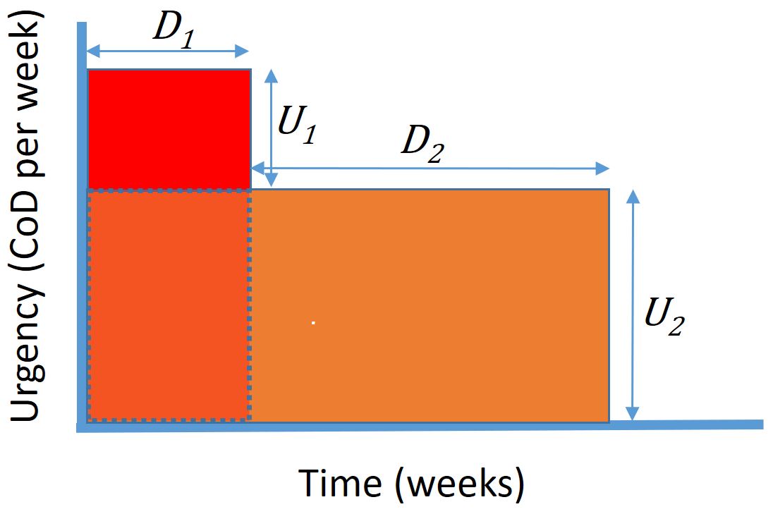
Part 1: Understanding Cost of Delay and its Use in KanbanIn Part 3 we established why the factor used for prioritising work items is urgency divided by the development delay (U/D). The item to be done first should have the highest value for this term (sometimes referred to as the "wisjif" or CD3). Urgency is the rate of decay of the business value (the Delay Cost per week) and we must estimate both the business value and Delay Cost Profile to derive this. In this post however we focus on the other variable. What is the appropriate value to use for D?
Part 2: Delay Cost and Urgency Profiles
Part 3: How to Calculate WSJF
Part 4: WSJF - Should you divide by Lead Time or Size? (this article)
Part 5: A "Qualitative" Formula for WSJF?
Part 6: Time is an Asset - Delay is a Cost
OK I'm going to tell you my conclusion before looking at why. It's a surprising conclusion (at least for me). My conclusion is that you should use "size", or a proxy for size like the estimated number of "user stories" in the work item, rather that the period of time before the item is released (Customer Lead Time). Mmm... if that's surprising to you (or if you've no idea why it might be surprising) read on!
Why use "size" rather than Customer Lead Time in WSJF?
To me the "first-glance" obvious answer to the question "What is D?" is Customer Lead Time. The business value is not realised until the item is delivered and "live". So the delay we are talking about is the time from the decision to implement (known as the commitment point in Kanban) to the release date; in other words, the Customer Lead Time. Some people have suggested that an estimate of the "size" of the item in some units (such as number of stories or story points) is an effective proxy for Lead Time. In fact it is a very poor proxy for this. (See for example Ian Carroll's blog [6] looking at correlation between size and Lead Time. The correlation is very weak, possibly non-existent.) The reason for this is low Flow Efficiency - the ratio of time working on an item to elapsed time. If Flow Efficiency is in single figures (typical for many teams) it is not surprising that size does not correlate well with Lead Time. Therefore we can't use size as a proxy for Lead Time. So why did I conclude that size is the correct divisor for wisjif?
Let's go back to the derivation of WSJF in the previous article (How to Calculate WSJF). The assumptions we used were that: the urgency was constant over the period of interest; and importantly, that the team's WiP limit was 1. Basically we assumed the second feature had to wait until the first feature had been delivered before we started on the next feature. In these circumstances the delay, is equal to Customer Lead Time - both for the wait until benefit occurs and for how long the previous item holds up the product team before it can start the next item. In reality these are two different wait times - provided that the WiP limit is allowed to be greater than one. The delay before benefit occurs is still the Customer Lead Time (let's call this T), but the team is held up by less that the Customer Lead Time - they can work on another work item while the first item is held up by a blocker or waiting for release. This is a much more realistic assumption than WiP=1 provided what we are talking about is a product feature, not a project.
This change in assumption changes the equation for the value realised by implementing item 1 followed by item 2. In the previous article we found this to be:
Now we are considering that the time during which the team is held up, is a different and shorter time than the time before the value is realised. Let's say the teams working on this product have capacity to deliver "stories" at an average rate of C stories per week. and that the estimated number of stories in the two work items are s1 and s2.
So the amount of time that the second item is held up by the first item is s1/C. The rest of the Customer Lead Time, T, is waiting time - let's call that w. So...

The value realised from item 1 followed by item 2 is now seen to be:
Again subtracting this same formula with the order of the items reversed (and seeing most of the terms cancel out), gives us the difference in value between the alternative orderings, as:

We can see from this formula that it is the term urgency divided by size for the 2 items (U/s) that determines which order is best. We do not need estimates of lead times for the items to find the optimum order for the work items.
See important note on assumptions below.
What if the "urgency" is not a constant?
What about the other important assumption in the simple WSJF formula - that the Urgency (Delay Cost per week) is a constant? In general, Urgency is not constant for work items over the whole period that there is still value in implementing them. However this does not matter if the Urgency is constant during the period that the competing items to be ordered will be implemented. In this case we can just go ahead and use the formula.
For "Fixed Date" items the formula is not appropriate. The determinant for when Fixed Date items should be started is the "last responsible moment", taking into account uncertainty in Customer Lead Time, and the degree of risk that is acceptable to the customer. The determinant for whether Fixed Date items should be started is the total value of the item, compared with the loss of value that occurs by delaying the next highest item to be prioritised. Usually we can just start Expedite items immediately and Fixed Date items before the last responsible moment without the need for estimation or calculation, making WSJF important only for the ordering of Standard items.
Intangible items would not be selected at all if we only applied the WSJF formula, since their immediate urgency is low. Nevertheless it is helpful to always include some Intangible items in the schedule for flexibility (if customer SLAa are threatened), and for preparation for future events. Policies around the use of Intangible items can be tuned to the business context and strategy.
In the next blog in this series we will consider some conclusions from this analysis of Cost of Delay and WSJF. Why is it important? When is it applicable? What to do when it is not applicable or not calculable?
Important Note on Assumptions (continuous delivery or batch)
The algebra above assumes that the waiting time part of the delay (w) does not vary for a given work item, regardless of whether it is implemented before or after another item. This is probably a reasonable assumption if these are "features" which are released as soon as they are completed, in some kind of continuous delivery process. If a batch delivery process is used (e.g. a release every 2 months), the delay is identical for features in the same batch. It would be wasteful to use WSJF for features within the same batch. The issue is which batch the feature is put in and this analysis probably needs to be more sophisticated (or simply qualitative rather than quantitative - see for example [7]) - to ensure items are in the right batch.
Read part 5: A "Qualitative" Formula for WSJF?
Back to part 1: Understanding Cost of Delay and its Use in Kanban